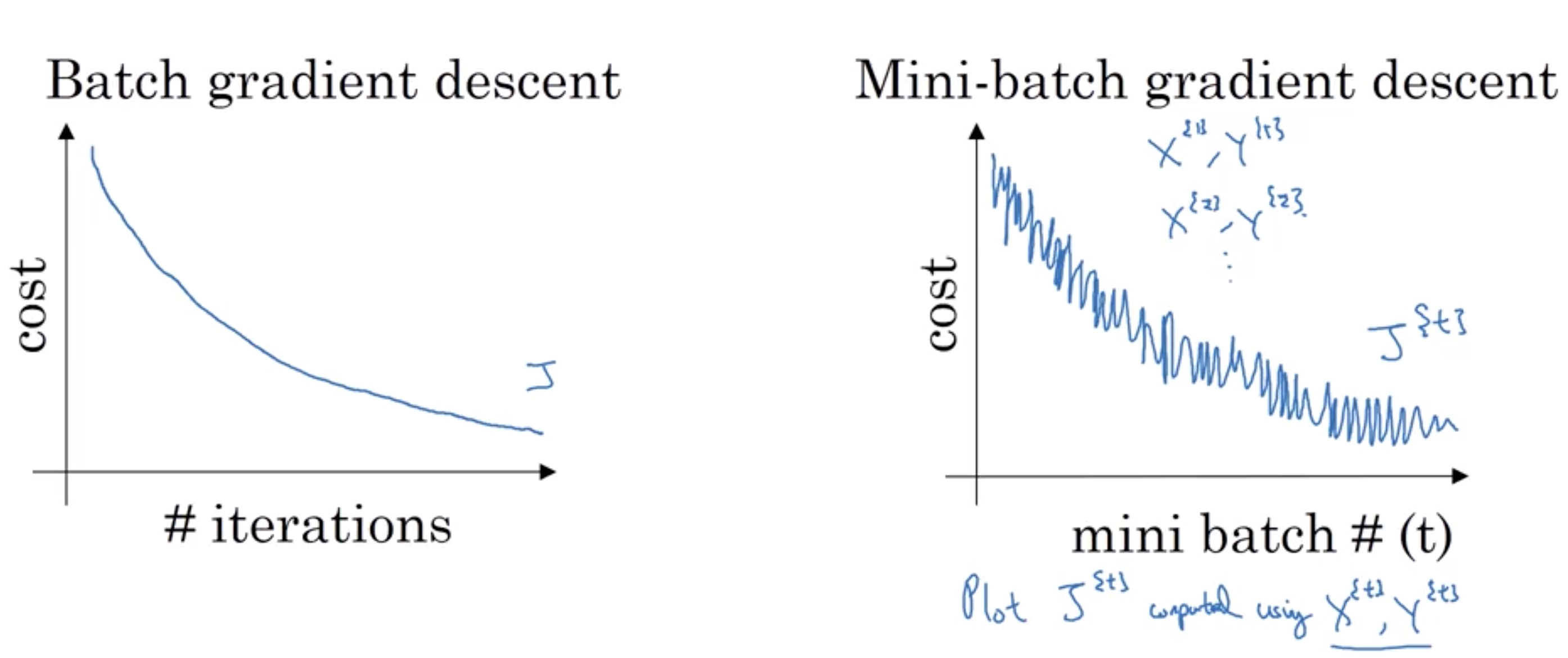
This week’s topic is about speeding up the learning process.

Mini batch

epoch: a single run through the whole training examples. If we are using mini batch technique with T batches, we will run T times of gradient descent wheras without mini batch, we will get only 1 time of gradient descent.

Notation

$$ a^{[l]\{t\}(m)} $$ means the the activation value of m examples in t minibatch in lth layer.

How to choose the size for each batch?

Recall in the previous note when we implement a deep nn with all the examples stack up to a matrix, it is actually a indicating we are using m as the mini batch size. Here we introduce 2 types of batch:

1. stochastic gradient descent: the size of each batch is 1.
2. batch gradient descent: 1 < batch size <= m

Choose 2^6, 2^7, 2^8 in practice.

Choosing a right batch size is vital for cost function to fall down to local optimal. This lead to another optimization technique taught by andrew called momentum.

Gradient descent with momentum

Suppose we have a huge amount of time series dataset

$$ (1-\beta)^{1\over\beta} ={1 \over \exp} $$ this is saying we are decaying $$ {1\over\beta} $$ units of previous average data as the current value.

v = 0
beta = 0.9 # adjust the value of beta for tuning how many days you want as your time window.
for i in range(1, len(examples)):
    v = beta * v + (1-beta)*examples[i-1]

this is just an estimation for calculating the average value in the previous $$ {1\over\beta} $$ units. $$ \begin{array}{l}{v_{d W}=\beta v_{d W}+(1-\beta) d W} \\ {v_{d b}=\beta v_{d b}+(1-\beta) d b} \\ {W=W-\alpha v_{d W}, \quad b=b-\alpha v_{d b}}\end{array} $$ the larger $$ {v_{d W}=\beta v_{d W}+(1-\beta) d W} $$ this term is, the greater the oscillation the gradient descent will get. Otherwise, the lesser. When beta is 0, this equation is actually traditional gradient descent.

What is the relationship between beta and the gradient descent?

Problems

For i = 0, 1, 2 … which in the early stage, the estimated value will cause large bias from the actual value. Since we have $$ v_{t}=\beta v_{t-1}+(1-\beta) \theta_{t} $$, for t == 0, we have v = 0. To avoid this, we let $$ v \over (1-\beta^{t}) $$

This whole process is actually called Exponentially weighted averages or exponentially moving averages. We can apply this to gradient descent. This is how momentum work, to avoid huge oscillations due to the large value of learning rate. !(source code of implementation here)[]

RMSprop(root mean square prop)

apply the

Adam optimization

combine momentum and RMSprop and bias correction together.

Hyperparameter choise:

alpha = # need to be tuned
beta1 = 0.9
beta2 = 0.99
epsilon = 10 ** (-8)

Learning rate decay

reduce learning rate alpha gradually for converge to local optimal.

Problem with local optima

andrew claim we don’t need to worry about the bad local optima problem for nn.